I have been captivated by creative coding and generative art for a while. After discovering some of the work by Antonio S.Chinchón and his blog Fronkonstin on using R and mathematics to create amazing art work, I decided to play around. Schotter (1968) is a famous piece by Georg Nees, a pioneer in computer graphics and probably one of the first creative coders.
To pay tribute to Georg, I decided to implement a chunk of code that would reproduce Schotter using R. There are probably several ways to code this algorithm and I am sure several people have done this before. My goal was to see if my current R knowledge could be use to program Schotter without checking other implementations and learn something on the way.
Here my thought process.
The libraries
Nowadays I use ggplot2 for every visualization, so I decided to utilize its amazing graphical powers. I also used dplyr although we could easily not use it here.
Building a square
The easiest way to build a square in ggplot2 is probably using geom_rect, however I did not find a way to rotate the geometry, so I decided to go for a polygon (geom_polygon) and control the position of the 4 vertices outside ggplot. For that I created the following function:
square<-function(x0=1,y0=1, size=1, angle=0){
  xor<-x0+size/2 #X origin (center of the square)
  yor<-y0+size/2 #Y origin (center of the square)

  tibble(
    x=c(x0,x0+size,x0+size,x0),
    y=c(y0,y0,y0+size,y0+size)
  )%>%mutate(x2=(x-xor)*cos(angle)-(y-yor)*sin(angle)+xor, #For rotation
             y2=(x-xor)*sin(angle)+(y-yor)*cos(angle)+yor) #for rotation
}
Where x0 and y0 control the position of lower left (or other depending on the axis orientation) vertex, size the length of the sides and angle the amount of rotation from the original position. An x and y for each vertex is set as a template relative to x0, y0 and size. In this way, we will be able to control the position of the square in the canvas. x2 and y2 are set as the rotated coordinates for x and y, respectively. Ultimately, we will use x2 and y2, that will be equal to x and y if angle is 0. I decided to generate new columns for the rotations so I can plot both, the original x, y and the rotated (I confess I had to brush up my trigonometry and google a few things for this).
ggplot(square())+
  geom_polygon(aes(x=x, y=y))+
  coord_fixed()# just so that axis are equally spaced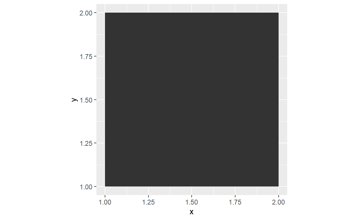
We have our first square!! We can now play with fill and color
ggplot(square())+
  geom_polygon(aes(x=x, y=y), fill=NA, color='black')+
  coord_fixed()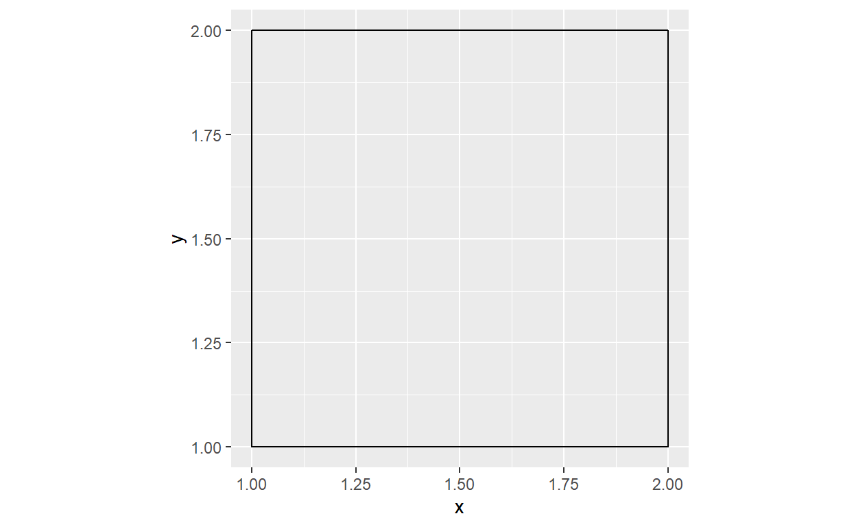
Let’s play with some parameters
ggplot(square(size=2,angle=pi/4))+#size 2 and rotate 45 degrees
  geom_polygon(aes(x=x, y=y), fill=NA, color='black')+
  geom_polygon(aes(x=x2, y=y2), fill=NA, color='red')+
  coord_fixed()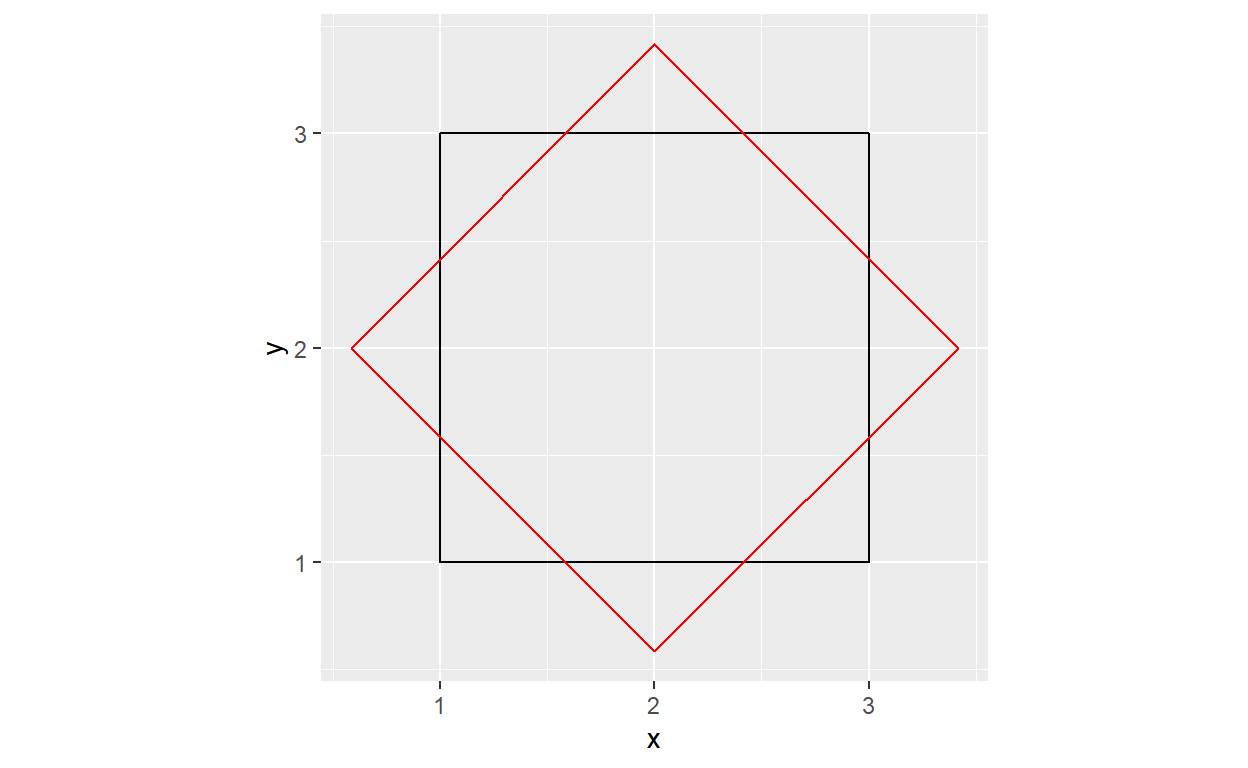
How many squares we want?
Schotter can be seen as a matrix of squares. A simple way to iterate through a matrix is to nest a loop inside a loop such that one loop goes through the rows and another through the columns.
The original Schotter has 12 columns and 24 rows (that I counted)
n<-24*12
df.list<-list()
  for (j in 1:24){ #iterate through the rows
    for (i in 1:12){ #iterate through the columns
      temp<-square(x=i, y=j) #create a square at column i and row j
      df.list[[n]]<-temp #save the data frame with the square n on a list
      n<-n-1
    }
  }
This chunk creates a data frame containing the x, y, x2 and y2 for 288 (24x12) squares, that we can plotted. To plot each square independently as we will need for later, we need to add a new geom_polygon layer for each square to a ggplot object. We could have done this in the previous loops, but in the course of this mini project I have learned that you can pass a list to ggplot. So, we can iterate though our list of square data frames using lapply and add a geom_polygon for each square (a bit slow on my friend).
ggplot() +
  lapply(df.list, function(square_data) {
    geom_polygon(data = square_data, aes(x = x2, y = y2), fill=NA, color='black')}
  )+
  coord_fixed()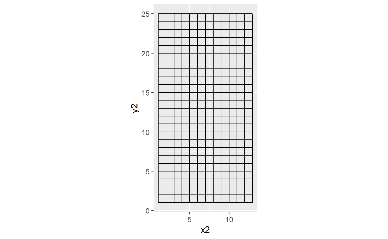
Now we have the grid of squares. At this point I have decided to deal with the unnecessary elements of the plot. I generated a theme function such that I can easily change the background color.
theme_background<-function(color='white'){
  theme(axis.ticks = element_blank(), axis.text = element_blank(),
        panel.background = element_blank(), panel.grid = element_blank(),
        plot.background = element_rect(fill = color),
        strip.background = element_rect(fill=color),strip.text = element_blank(),
        axis.title = element_blank(), legend.position = 'none')
}

ggplot() +
  lapply(df.list, function(square_data) {
    geom_polygon(data = square_data, aes(x = x2, y = y2), fill=NA, color='black')}
  )+
  coord_fixed()+
  theme_background()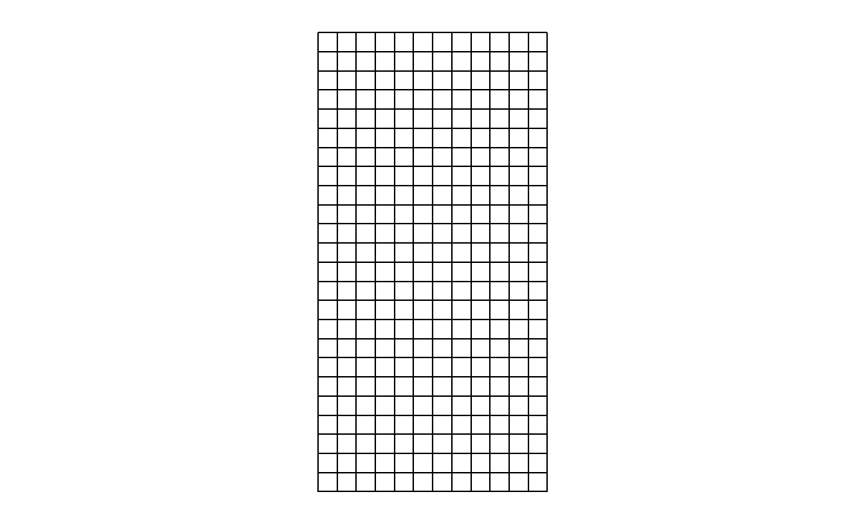
Generative process
Generative art is define by wikipedia as:
Generative art refers to art that in whole or in part has been created with the use of an autonomous system. An autonomous system in this context is generally one that is non-human and can independently determine features of an artwork that would otherwise require decisions made directly by the artist. An easy way to give autonomy to our code is by introducing randomness. As we can appreciate from Schotter, both the position and the angle of the squares seems to be more random and move away from the ‘calm’ stage as we move through the rows. We will add this to our nested loops by generating a random displacement and rotation for each square that increases by row.
n<-24*12
df.list<-list()
  for (j in 1:24){ #iterate through the rows
    for (i in 1:12){ #iterate through the columns
      displace<-runif(1,-j,j) #a random number is generated from a uniform distribution with min=-j and max=j
      rotate<-runif(1,-j,j) #random number to rotate the square
      temp<-square(x=i+displace, y=j+displace, angle=rotate) #create a square at column i and row j displaced by displace
      df.list[[n]]<-temp #save the data frame with the square n on a list
      n<-n-1
    }
  }

ggplot() +
  lapply(df.list, function(square_data) {
    geom_polygon(data = square_data, aes(x = x2, y = y2), fill=NA, color='black')}
  )+
  coord_fixed()+
  theme_background()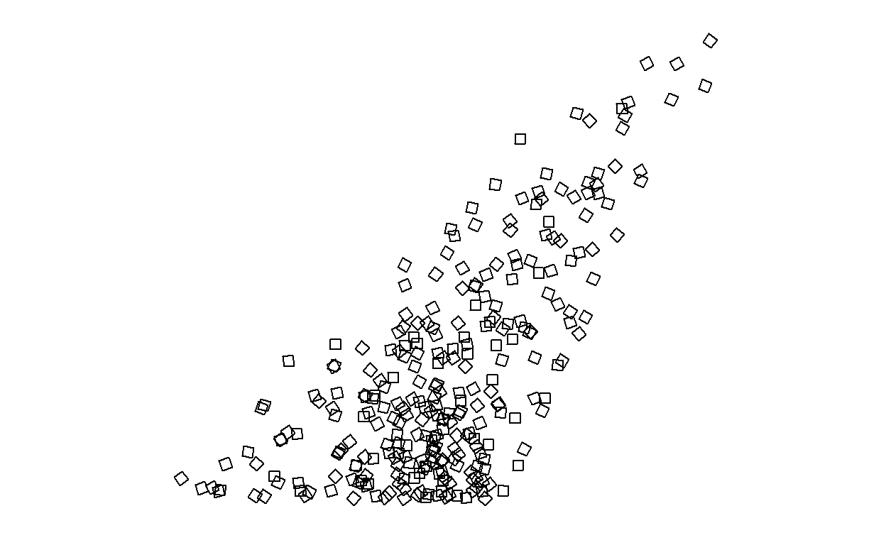
Ups! Something isn’t quite right (although I like it!). I think is because j, that controls how much displacement and rotation can be added get to be too big in respect to x and y. So, let’s control for that. For that I divided j by 40 in the case of displace and by 100 in the case of rotate. I found these numbers by playing around. I also flipped y axis.
n<-24*12
df.list<-list()
  for (j in 1:24){ #iterate through the rows
    for (i in 1:12){ #iterate through the columns
      displace<-runif(1,-j/40,j/40) #a random number is generated from a uniform distribution with min=-j and max=j
      rotate<-runif(1,-j/100,j/100) #random number to rotate the square
      temp<-square(x=i+displace, y=j+displace, angle=rotate) #create a square at column i and row j displaced by displace
      df.list[[n]]<-temp #save the data frame with the square n on a list
      n<-n-1
    }
  }

ggplot() +
  lapply(df.list, function(square_data) {
    geom_polygon(data = square_data, aes(x = x2, y = y2), fill=NA, color='black')}
  )+
  coord_fixed()+
  theme_background()+
  scale_y_reverse()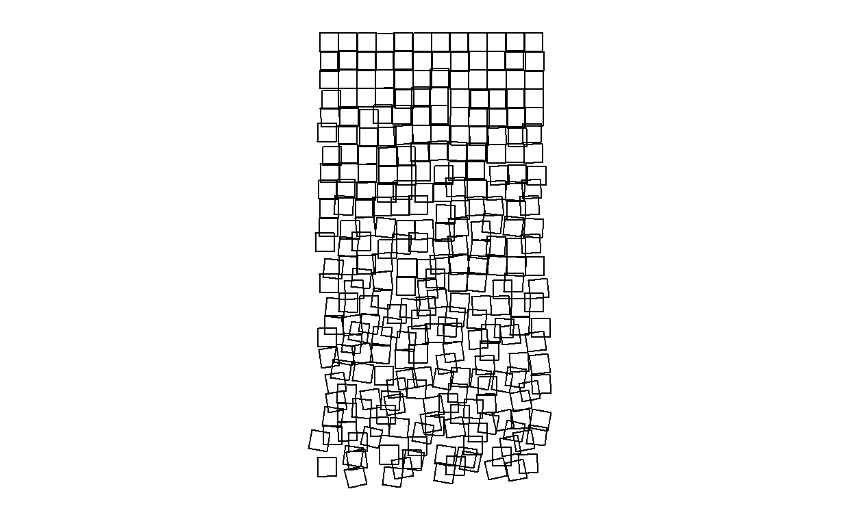
And voila! we have coded a generative algorithm to produce something like Schotter. Because the randomness, every time we run the code, the result will be different.
Now we wrap the code in a function so that we can easily change parameters
Schotter<-function(ncol_s=12, nrow_s=24, control_dis=40,
                   control_rot=100, fill_s=NA, color_s='black', alpha_s=0.2,
                   back_color='white'){
n<-ncol_s*nrow_s
df.list<-list()
  for (j in 1:nrow_s){
    for (i in 1:ncol_s){
      displace<-runif(1,-j/control_dis,j/control_dis)
      rotate<-runif(1,-j/control_rot,j/control_rot)
      temp<-square(x=i+displace, y=j+displace, angle=rotate)
      temp$s<-rep(n)
      df.list[[n]]<-temp
      n<-n-1
    }
  }

ggplot() +
  lapply(df.list, function(square_data) {
    geom_polygon(data = square_data, aes(x = x2, y = y2),
                 alpha=alpha_s, fill=fill_s, color=color_s)}
  )+
  theme_background(color = back_color)+
  coord_fixed()+
  scale_y_reverse()
}
We can now play!
Schotter()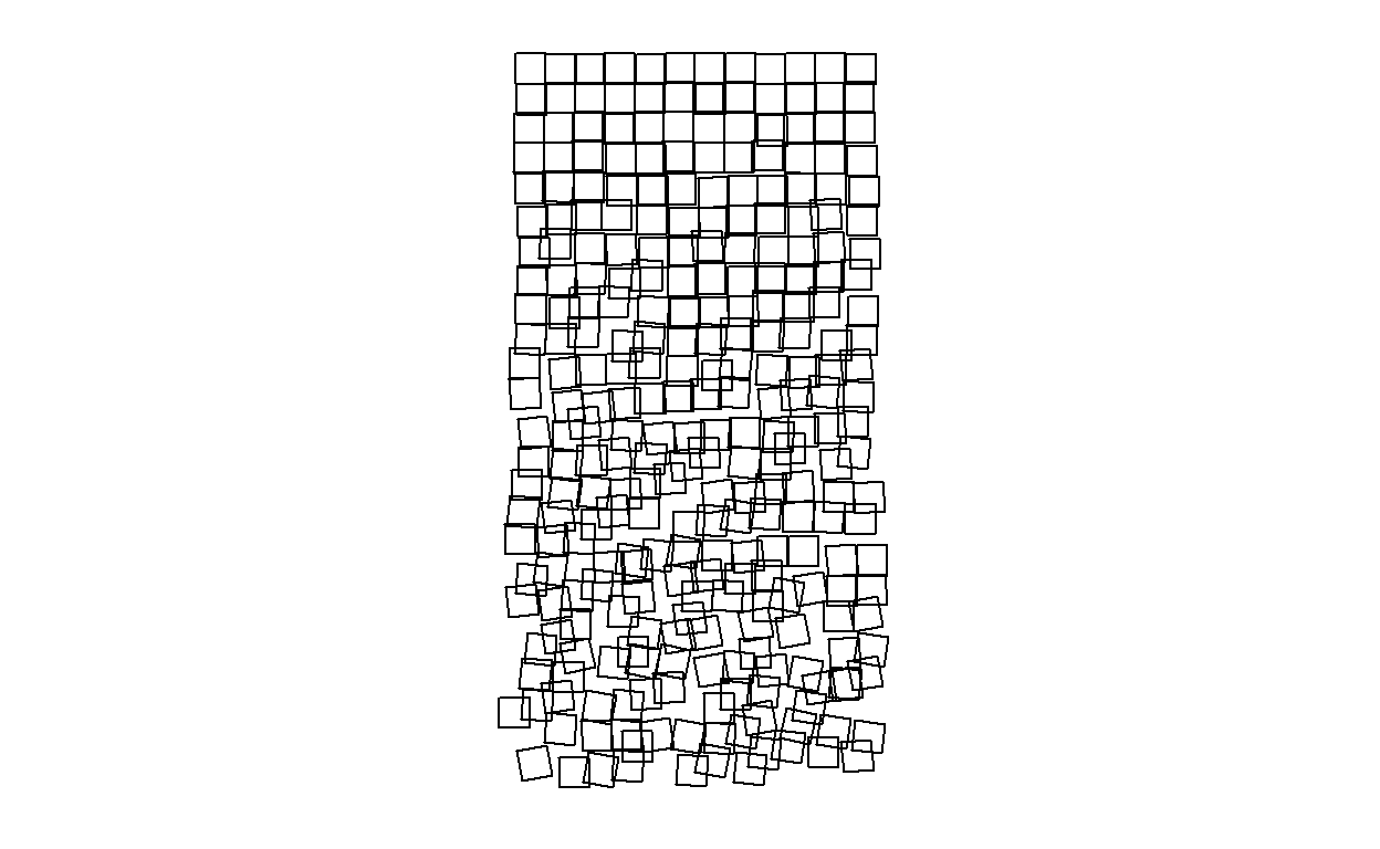
Schotter(fill='firebrick', color='orange', nrow_s = 48, control_dis = 20)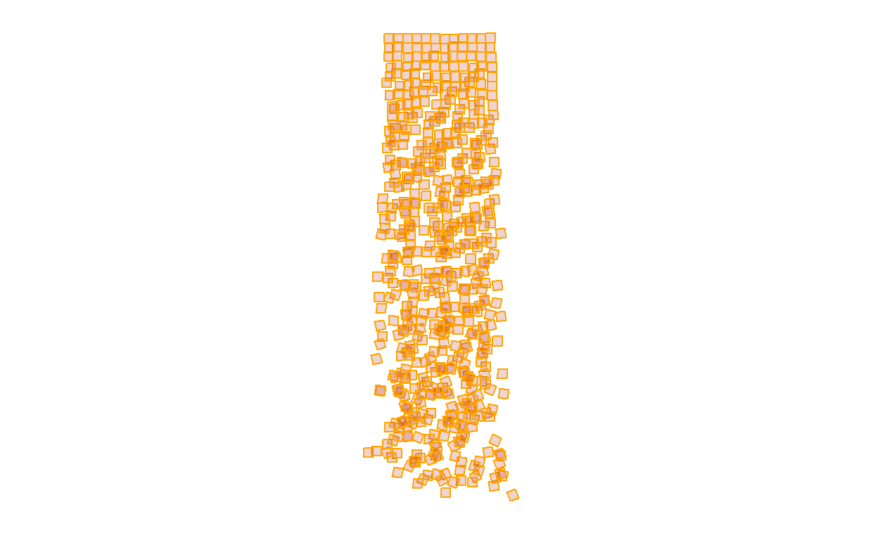
The End
This is all for now. There are a few ways the code could be improved, but I am happy with the result and I have had fun and learned something new!