This post will show you how you can extract and visualize your network of co-authors. You can also find the code for this post on GitHub.
Luckily for us, the hard work needed for this has been already programmed by amazing people out there, so we will be using these packages:
Extracting Pubmed information
The easyPubMed package can be used for… yes, you guessed right… easily extract information from Pubmed. So, the first thing to do is to search us and extract the list of authors in our papers from the ‘medline’ format, tagged as ‘AU’.
my_entrez_id <- get_pubmed_ids('Torres-Espin A')
my_author_txt <- fetch_pubmed_data(my_entrez_id, format = "medline")
authors<-my_author_txt[str_detect(my_author_txt, "^AU ")]
coauthors_list<-unique(str_remove_all(authors, '^AU  - '))
head(coauthors_list)

sort(coauthors_list)
Note that we use unique because we might have more than one paper with the same author. We do this because now we are going to search the list of co-authors to get the relationship of publication between them. If you only want to get the first level connections of each co-author with you, then do not need to collapse the coauthors_list.
Now let’s create a data frame containing the list of co-authors for each author on our list of co-authors. We can do that by iterating through the same code we did before and saving the results in a list of data frames. We will stack the list of data frames at the end by calling rbind. If you know some R you probably know that this code can be collapsed in fewer lines and be more efficient using apply. I like using loops from time to time!
author_list<-list()#define the list to save the data frames

for (i in 1:length(coauthors_list)){
  my_entrez_id <- get_pubmed_ids(coauthors_list[i])
  my_author_txt <- fetch_pubmed_data(my_entrez_id, format = "medline")

  if (length(my_author_txt)==0) next()

  authors<-my_author_txt[str_detect(my_author_txt, "^AU ")]
  authors<-str_remove_all(authors, '^AU  - ')
  author_list[[i]]<-data.frame(co_authors=authors, author=coauthors_list[i])
}
author_df<-do.call(rbind, author_list)#stack data frames
We can save this for later use so that we do not need to do the search again!
saveRDS(author_df, "author_df.Rds")The next step is filtering our data frame to keep only the co-authors of our co-authors that are also our co-authors (this is getting tricky…). You could leave the co-authors of your co-authors that you have not published with, but that can make the graph quite big and not useful for plotting. After filtering we create a new variable with the joint string between co-author and author, so that we can count how many times that joint happens.
author_df<-author_df[author_df$co_authors%in%author_df$author,]%>%
  mutate(co_authors = ifelse(co_authors =="Torres Espin A", "Torres-Espin A", co_authors),
         author = ifelse(author =="Torres Espin A", "Torres-Espin A", author))%>%
  mutate(co_edge=paste(co_authors, author, sep = '_'))%>%
  group_by(co_edge)%>%
  summarise(count=n())%>%
  separate(co_edge, c('co_authors','author'),sep = '_')

author_df<-author_df%>%
  group_by(co_authors, author)%>%
  summarise(count = sum(count))
We are ready to create the graph from the data frame. We specify the weight of the edges (using E) as the count of the times two authors published together. Note that in our count data ‘author 1-author 2’ counts different than ‘author 2-author 1’ for the same paper, so we are counting each article twice. That is not a problem since we are considering a undirected graph. We just need to remember that we will be representing each article 2 times. I did not care because graphically does not matter. Now, we plot the graph (very rough!)
author_g<-graph_from_data_frame(author_df,directed = F)
E(author_g)$weight<-author_df$count
author_g<-simplify(author_g)
#layout_nicely(author_g)
plot(author_g)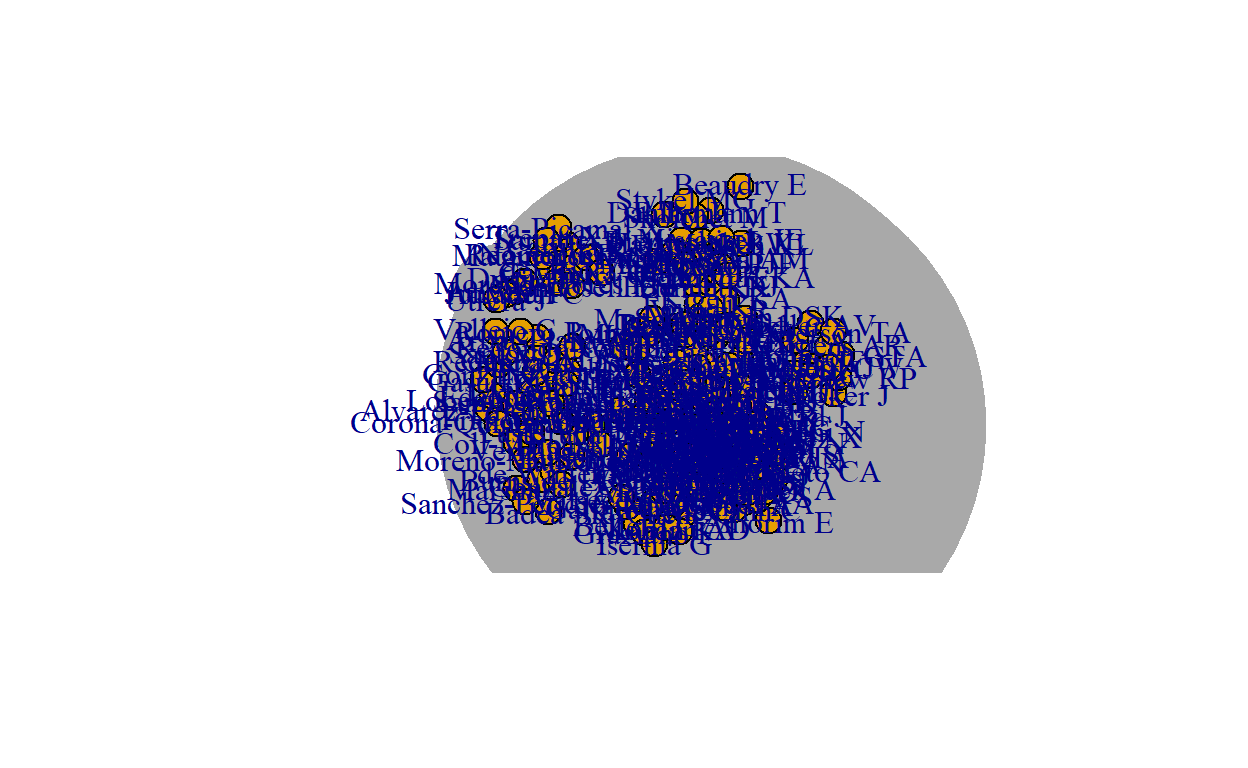
Last step is to make the graph pretty and play with the parameters.
For a good network visualization tutorial in R check [this post]( https://mr.schochastics.net/material/netvizr/)UPDATE
I decided to use the networkD3 package for computational efficiency. In the initial version of this post I used the visNetwork package, which I find an amazing tool, so I recommend you explore it if you use networks.
group<-rep(1, length(V(author_g)))
group[377]<-2

author_d3 <- igraph_to_networkD3(author_g, group = as.character(group))

forceNetwork(Links = author_d3$links, Nodes = author_d3$nodes,
             Source = 'source', Target = 'target', NodeID = 'name',
             Group = "group", linkColour = "lightgrey",
             colourScale =JS('d3.scaleOrdinal().domain(["1", "2"]).range(["#ADD8E6", "#FF6600"])'),
             opacity = 0.9)
Code from initial post
vis_g<-toVisNetworkData(author_g) #coverts the igraph object to visNetwork
vis_g$edges$value<-vis_g$edges$weight #specify the values for eadges as the weights (number of papers for pairs)

#vis_g$nodes$title<-co_authors_abel$author_name #name of the nodes

#plot the network
visNetwork(nodes = vis_g$nodes, edges = vis_g$edges, height = "400px", width = '500px')%>%
  visNodes(size = 10, shape='cicle', mass=2,font=list(color='white'),fixed = F) %>%
  visEdges(length = 10,physics = T, smooth = list(enabled=T))%>%
  visLayout(randomSeed = 666)%>%
  visOptions(highlightNearest = list(hover = T),
             nodesIdSelection = list(enabled = TRUE))%>%
  visPhysics(stabilization = T, minVelocity = 10, maxVelocity = 25)
Or we can use the ggnetwork package for static networks. It is much faster to plot and integrates with ggolot2!
network<-ggnetwork(author_g, layout = igraph::layout.fruchterman.reingold(author_g))
network<-network%>%
  group_by(name)%>%
  mutate(node_size = n())

ggplot(network,
       aes(x = x, y = y, xend = xend, yend = yend)) +
  geom_edges(size = 0.6, color = "grey50", curvature = 0.1, alpha= 0.1,
             show.legend = F) +
  geom_nodes(aes(size = node_size),show.legend = F, color = "black",
             fill = "steelblue1",
             shape = 21) +
  # geom_nodelabel(aes(label = name, fill = group), size = 2)+
  # geom_nodes(aes(size = weight+weight*2), show.legend = F, color = "steelblue", alpha = 0.5) +
  theme_blank()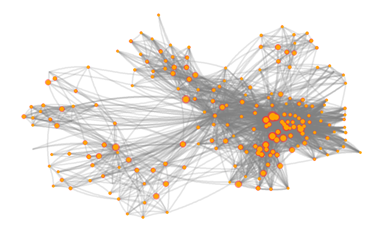
ggsave("network_points.png", width = 15, height = 10)DONE!
Now you can save the network as html using the saveNetwork function. For the network in my co-authors section, I did some extra processing steps to consider that some times same author might publish with slightly different names. I also added some groups and colors. I would let you be creative.